Transformer Models

Motivating the Transformer Model

• An RNN has $3$ problems stemming from their sequential architecture:

  • Information loss

    • Although GRU/LSTM mitigates the loss, the problem still exists

  • Suffers from the vanishing gradient problem

    • Specifically, the problem caused by longer input sequences

  • Enforces sequential processing of hidden layers

    • Parallelizing RNN computations is nearly impossible

• The more words we have in our input sequence, the more time it takes decode the sequence

  • The number of steps is equal to $T_{y}$

• Whereas, transformers support the following benefits:

  • Information loss isn't a problem

    • Since, attention scores are computed in a single step

  • Don't suffer from the vanish gradient problem

    • Specifically, the problem caused by longer input sequences
    • This is because there is only one gradient step

  • Doesn't enforce sequential processing of hidden layers

    • Parallelizing these computations is much easier
    • Since, they don't require sequential computations per layer
    • Meaning, they aren't dependent on previous layers

Describing the Basics of a Transformer

• A transformer uses an attention mechanism without being an RNN
• In other words, it is an attention model, but is not an RNN
• A transformer processes all of the tokens in a sequence simultaneously
• Then, attention scores are computed between each token
• A transformer doesn't use any recurrent layers
• Instead, a transformer uses multi-headed attention layers

Introducing the Architecture of a Transformer

• A transformer consists of $3$ basic components:

  • Positional encoding functions
  • Encoder
  • Decoder

Defining Positional Encoding Functions

• An input embedding maps a word to a vector

• However, the same word in a different sentence may carry a new meaning based on its surrounding words:

  • Sentence 1: I love your dog!
  • Sentence 2: You're a lucky dog!
• This is why we use positional encoding vectors

• A positional encoding vector adds positional context to embeddings

  • It adds context based on the position of a word in a sentence

$$PE(pos, 2i) = \sin(\frac{pos}{10000^{\frac{2i}{d_{model}}}})$$

• Where the formula has the following variables and constants:

  • $pos$ is the position of a given word in its sentence
  • $i$ is the index of the $i^{th}$ element of the word embedding
  • $d_{model}$ is the size of the word embedding
• The following is an example of applying the positional encoding function to the $4$-dimensional word embedding of dog:

$$\underbrace{\begin{bmatrix} 0.3 \\ 0.4 \\ 0.7 \\ 0.1 \end{bmatrix}}_{\text{embedding of dog}} + \quad \boxed{\text{positional encoding}} \; = \; \underbrace{\begin{bmatrix} 0.4 \\ 0.6 \\ 0.8 \\ 0.9 \end{bmatrix}}_{\text{positional encoding of dog}}$$

Initial Steps of the Encoder

• So far, we've completed the following steps, including:

  • Embedding our input
  • Performing positional encoding on the embedding
• Now, we're ready to pass the positional encoding into the encoder

• This includes performing the following specific steps:

  • Multi-head attention
  • Normalization
  • Feed-forward
• Before introducing multi-head attention, let's first start off by defining self-head attention

Types of Attention in Neural Networks

• There are $3$ general types of attention:

  • Encoder/decoder attention
  • Causal self-attention
  • Bi-directional self-attention
• For encoder/decoder attention, a sentence from the decoder looks at another sentence from the encoder
• For causal attention, words in a sentence (from an encoder or decoder) look at previous words in that same sentence
• For bi-directional attention, words in a sentence (from an encoder or decoder) look at previous and future words in that same sentence
• Neither of these attention mechanisms are mutually exclusive
• Meaning, any attention layer can incorporate any of the $3$ types of attention

Introducing Self-Head Attention in the Encoder

• Attention is how relevant the $i^{th}$ word in the input sequence relative to other words in the input sequence
• Self-attention allows us to associate it with fruit in the following sentence:

$$\text{The fruit looks tasty and it looks juicy}$$

• When calculating attention, there are $3$ components:

  • A query matrix $Q$, consisting of query vectors $q_{i}$

    • $q_{i}$ represents a vector associated with a single input word

  • A key matrix $K$, consisting of key vectors $k_{i}$

    • $k_{i}$ represents a vector associated with a single input word

  • A value matrix $V$, consisting of key vectors $v_{i}$

    • $v_{i}$ represents a vector associated with a single input word
• Specifically, each individual matrix is the result of matrix multiplication between the input embeddings and $3$ matrices of trained weights:
• These $3$ weight matrices include $W_{Q}$, $W_{K}$, and $W_{V}$

• Again, $q_{i}$, $k_{i}$, and $v_{i}$ refer to identical words of a sequence

  • However, the values associated with $q_{i}$, $k_{i}$, and $v_{i}$ are different
  • This is because $W_{Q}$, $W_{K}$, and $W_{V}$ are weight matrices learned during training
• The formulas for $q_{i}$, $k_{i}$, and $v_{i}$ are defined below:

$$q_{1} = x_{1} \cdot W_{Q} \\ k_{1} = x_{1} \cdot W_{K} \\ v_{1} = v_{1} \cdot W_{V}$$

• The example below has the following properties:

  • Translating a sentence with $2$ words: hello and world

  • Each word embedding vector has a length of $e_{n} = 4$

    • Implying, there are $4$ words in our vocabulary

  • Each $W_{Q}$, $W_{K}$, and $W_{V}$ is a $e_{n} \times m$ matrix

    • Where, $m$ is an adjustable hyperparameter
    • For now, we'll decide to assign $m = 3$
  • Each $q_{i}$, $k_{i}$, and $v_{i}$ has a length of $m$

• Notice, $q_{1}$ is the result of multiplying $x_{1}$ and $W_{Q}$ together
• Notice, $k_{1}$ is the result of multiplying $x_{1}$ and $W_{K}$ together
• Notice, $v_{1}$ is the result of multiplying $x_{1}$ and $W_{V}$ together

Steps for Calculation Self-Attention in the Encoder

• At a high level, a self-attention block does:

  1. Start with trained weight matrices $W_{Q}$, $W_{K}$, and $W_{V}$

  2. Compute embeddings to determine how similar $X$ or previous activations are to input words and output words

     • Roughly, $Q$ represents embeddings of output words
     • Roughly, $K$ and $V$ represent embeddings of input words
     • In other words, $Q$ learns patterns from our output sentence
     • And, $K$ and $V$ learns patterns from our input sentence

  3. Convert these similarity scores to probabilities

     • This is because probabilities are easier to understand

• At a lower level, a self-attention block does:

  1. Receives trained weight matrices $W_{Q}$, $W_{K}$, and $W_{V}$

  2. Computes $Q$, $K$, and $V$:

     • $Q = X \cdot W_{Q}$
     • $K = X \cdot W_{K}$
     • $V = X \cdot W_{V}$

  3. Computes alignment scores by $q_{i} \cdot k_{j}$

     • Here, we're looking for keys $k_{j}$ (input words) that are similar with our query $q_{i}$ (output word)
  4. Divide alignment scores by $\sqrt{d_{k}} = \sqrt{4}$ for more stable gradients

  5. Pass values from our previous step through a softmax function

     • This formats each alignment score as a probability

  6. Compute dot product of $v_{i} \cdot \text{softmax value}$ to get $Z$ matrix

     • Here, $Z$ represents our attention scores
     • Roughly, $V$ represents how similar words from $Q$ and $K$ are
     • Multiplying softmax values by $V$ represents weighting each value $v_{j}$ by the probability that $k_{j}$ matches the query $q_{i}$

Understanding Dimensions of $Q$, $K$, and $V$

• Suppose we're translating an English sentence to a German sentence

• $Q$ has the following dimensions:

  • Number of rows $=$ number of words in the German sentence $L_{Q}$
  • Number of columns $=$ a proposed length $D$ of the embedding

• $K$ has the following dimensions:

  • Number of rows $=$ number of words in the English sentence $L_{K}$
  • Number of columns $=$ a proposed length $D$ of the embedding

• $V$ has the following dimensions:

  • Number of rows $=$ number of words in the English sentence $L_{K}$
  • Number of columns $=$ a proposed length $D$ of the embedding

• $A=\text{softmax}(QK^{T})$ has the following dimensions:

  • Number of rows $=$ number of words in the German sentence $L_{Q}$
  • Number of cols $=$ number of words in the English sentence $L_{K}$

• $Z=AV$ has the following dimensions:

  • Number of rows $=$ number of words in the German sentence $L_{Q}$
  • Number of columns $=$ a proposed length $D$ of the embedding
• Here, $D$ is an adjustable hyperparameter
• Mathematically, these matrices are denoted as the following:

$$Q: L_{Q} \times D \\ K: L_{K} \times D \\ V: L_{K} \times D \\ A: L_{Q} \times L_{K} \\ Z: L_{Q} \times D$$

Calculating Self-Attention in the Encoder

• $q_{i}$, $k_{i}$, and $v_{i}$ are simply abstractions that are useful for calculating and thinking about attention

  • However, they are not attention scores themselves
  • Each row of $Q$, $K$, and $V$ are associated with an input word
  • Meaning, $q_{i}$, $k_{i}$, and $v_{i}$ refer to the $i^{th}$ input word
• For now, let's focus on calculating the attention scores for the first word $x_{1}$ relative to the other words in the sentence (i.e. $x_{2}$)

• To calculate attention scores, we just take the dot product of $q_{i} \cdot k_{j}$

  • This determines how relevant word $q_{i}$ is to word $k_{j}$

• The following diagram illustrates computing attention scores for:

  • $q_{1}$ and $k_{1}$
  • $q_{1}$ and $k_{2}$

• Next, we'll normalize the attention scores by:

  1. Dividing them by $\sqrt{d_{k}}$

     • This leads to having more stable gradients

  2. Then, passing those outputs through the softmax function

     • The softmax function formats values as probabilities
     • Thus, the output determines how much each word will be expressed for this input word $x_{1}$

  3. Computing the dot product of the softmax value and each $v_{i}$

     • This keeps relevant words and drowns out irrelevant words

• The steps can be condensed using matrix multiplication
• Thus, each row of $Z$ is a vector for each word
• Again, $Z$ represents the attention scores
• The following computes self-attention on $x_{1}$ and $x_{2}$:

Improving Self-Attention with Multi-Headed Attention

• The transformer paper refined the self-attention layer by adding a mechanism called multi-headed attention

• This improves the accuracy and performance of self-attention:

  • Accuracy: Different sets of $Q_{h}$, $K_{h}$, and $V_{h}$ can learn different contexts and patterns in the sentence

    • We'll know it refers to fruit here:
    $$\text{The fruit looks tasty and it looks juicy}$$
  • Performance: Simply splitting $Q$, $K$, and $V$ into smaller heads allows us to parallelize matrix multiplication and other computations on these heads

• Without using multi-headed attention, self-attention will weight always assign the most attention to itself

  • Consequently, it becomes useless
  • Which is why we include $8$ different sets of heads
  • Then, we'll be able to pick up on more interesting contexts
• Although additional sets of queries/keys/values are added, they can be processed in parallel with each other

• The number of sets of queries/keys/values are determined by the number of attention heads

  • This number is an adjustable hyperparameter
  • For future examples, we'll assign this number $h=8$, since this is the default number specified in the transformer paper
• The mult-headed attention mechanism follows the same steps as the steps in self-attention

• However, multi-headed attention layer makes a few adjustments:

  1. Receives trained weight matrices $W_{Q}$, $W_{K}$, and $W_{V}$

  2. Compute $h=8$ sets of $Q$, $K$, and $V$:

     • $Q = X \cdot W_{Q}$
     • $K = X \cdot W_{K}$
     • $V = X \cdot W_{V}$
  3. Computes attention scores by $q_{i} \cdot k_{j}$
  4. Divide attention scores by $\sqrt{d_{k}} = \sqrt{4}$ for more stable gradients
  5. Pass the values in the previous step through the softmax function
  6. Compute dot product of $v_{i} \cdot \text{softmax value}$ to get $Z$ matrix
  7. Stack the $8$ $Z$ matrices together
  8. Multiply stacked $Z$ matrix by another trained $W_{O}$ matrix $Z \cdot W_{O}$ to get $Z_{final}$

Defining the Masked Multi-Headed Attention Blocks

• The masked multi-headed attention block is essentially the same as an attention block
• However, the decoder must receive the information from the encoder
• Otherwise, we wouldn't have learned anything from the encoder

• Therefore, the masked multi-headed attention block receives:

  • Information from encoder: all of the words from the english sentence
  • Information from previous decoder layers: previous words in the translated sentence
• Thus, the masked multi-headed attention block masks upcoming words in the translated sentence by replacing them with $0$
• Then, the attention network won't use them

Training Multi-Headed Attention Blocks

• $Q$, $K$, and $V$ are trained and used in the encoder's multi-headed attention block

• Then, $K$ and $V$ are passed to the decoder's masked multi-headed attention block

  • In the multi-headed attention block, its own individual $Q$ is trained

• Lastly, the same $K$ and $V$ are passed again to the decoder's second multi-headed attention block

  • The masked multi-headed attention block passes its $Q$ to this multi-headed attention block
• This is a crucial step in explaining how the representation of two languages in an encoder are mixed together

• In summary, there are $2$ $Q$ matrices trained

  • One $Q$ is trained and used in the encoder
  • Another $Q$ is trained and used in the decoder

• And, there is only $1$ $K$ and $1$ $V$ matrix trained

  • They are trained and used in the encoder and decoder

Illustrating Multi-Headed Attention after Training

• After calculating each of the $8$ heads, we can refer to the attention heads relative to individual words to determine what each head focuses on
• In the following example, we encode the word it
• Notice, one attention head focuses most on the animal
• Another attention head focuses on tired
• In a sense, the model's representation of the word it bakes in some of the representation of both animal and tired

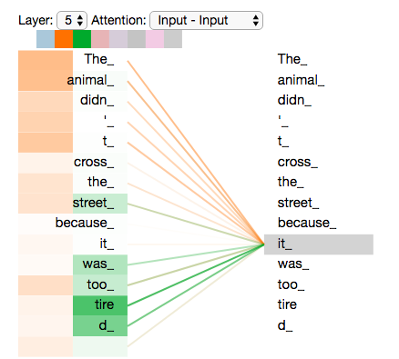
• In the above example, notice how we're only focused on the $2^{nd}$ and $3^{rd}$ heads
• By comparing particular heads with each other, we can get a decent idea about what other words each head focuses on relative to an individual word
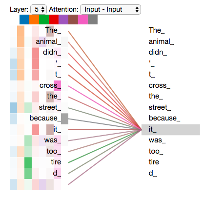
• Notice, if we focus on all of the heads, any analysis becomes less interpretable:

Illustrating the Encoder and Decoder during Training

• The input of the encoder is an input sequence
• The output of the encoder is a set of attention vectors $K$ and $V$
• These $2$ matrices are used by the decoders in its attention layers
• This helps the decoder focus on appropriate places in the input sequence
• Refer here for more detailed illustrations of the encoder and decoder

Applications of a Transformer Model

• Automatic text summarization
• Auto-completion
• Named entity recognition (NER)
• Question answering
• Machine translation
• Chat bots
• Sentiment analysis
• Market intelligence
• Text classification
• Character recognition
• Spell checking

Popular Types of Transformers

• GPT-3

  • Stands for generative pre-training for transformer
  • Created by OpenAI with pre-training in 2020
  • Used for text generation, summarization, and classification

• T5

  • Stands for text-to-text transfer transformer
  • Created by Google in 2019
  • Used for question answering, text classification, question answering, etc.

• BERT

  • Stands for bidirectional encoder represeentations from transformers
  • Created by Google in 2018
  • Used for created text representations

---

tldr

• The positional encoding vectors find patterns between positions of words in the sentences
• The attention layers find patterns between words in the sentences
• Normalization helps speed up training and processing time
• Multi-headed attention layers only involve to matrix multiplication operations

• Multi-headed attention improves both performance and accuracy:

  • Accuracy: More heads imply more detectable patterns between words
  • Performance: These heads can be computed and trained in parallel using GPUs
• Multi-headed attention scores are formatted as probabilities using the softmax function
• The fully connected feed-forward layer in the encoders and decoders are trained using ReLU activation functions

• Roughly, $Q$ represents embeddings of output words

  • $Q$ learns patterns from our output sentence

• Roughly, $K$ and $V$ represent embeddings of input words

  • $K$ and $V$ learns patterns from our input sentence
  • $V$ represents how similar words from $Q$ and $K$ are
• The encoder and decoder use the same $K$ and $V$
• The encoder and decoder has its own $Q$

---

References

• Stanford Deep Learning Lectures
• Stanford Lecture about LSTMs
• Lecture about Self-Attention in NLP
• Lecture about Multi-Headed Attention in NLP
• Lecture about Types of Attention in NLP
• Defining the Use and Architecture of Transformers
• Illustrating the Architecture of Transformers
• Paper about Transformer Models
• How Attention is Calculated During Training
• Intuition behind Positional Encoding Vectors
• Post about Positional Encoding Vectors
• Post about Attention Mechanism
• Detailed Description about Self-Attention
• Paper about Alignment and Attention Models