Approximate Matching

Motivating Matching for Causality

• The goal of any causal analysis is to isolate some causal effect

• To do this, we must satisfy the backdoor criterion in our study

  • Meaning, we must close all open backdoor paths
• Closing backdoor paths can be achieved through carefully performing conditioning strategies in our study

• Roughly, there are three different types of conditioning strategies:

  • Subclassification
  • Exact matching
  • Approximate matching

Motivating the Conditional Independence Assumption

• Conditional independence assumption (or CIA) states that a treatment assignment is independent of potential outcomes after conditioning on observed covariates

• Sometimes we know that randomization occurred only conditional on some observable characteristics

  • This would violate the backdoor path criterion

• In order to estimate a causal effect when there is a confounder, we must satisfy CIA

  • In DAGs notation, this refers to enforcing closed paths everywhere for confounders
  • Meaning, CIA implies there isn't any confounding bias

$$(Y^{1}, Y^{0}) \perp T | X$$

Introducing Matching for Estimating $ATE$

• Matching is one of three conditioning method used for satisfying the backdoor criterion
• Matching estimates $ATE$ by imputing missing potential outcomes by conditioning on the confounding
• Specifically, we could fill in missing potential outcomes for each treatment unit using a control group unit that was closest to the treatment group unit for some $X$ confounder
• This would give us estimates of all the counterfactuals from which we could simply take the average over the differences
• Specifically, matching ensures that CIA isn't violated

Using Matching instead of Subclassification

• Subclassification uses the difference between treatment and control group units and achieves covariate balance by using the $K$ probability weights to weight the averages
• As long as there is enough data for stratifying our covariates, subclassification can be a viable option
• However, if subclassification suffers from the curse of dimensionality, then we must use other methods (like matching)
• Typically, curse of dimensionality exists, so we'll prefer other methods like matching
• Specifically, subclassification is a weighting method used on all individuals, regardless of the overlap of distributions
• Whereas, matching is a form of stratification (or sampling method) that attempts the match distributions

Illustrating Approximate Nearest Neighbor Matching

• Exact matching can break down when the number of covariates $K$ grows larger than $1$
• Thus, we must estimate the closest covariate using distance measurements
• Sometimes, we have several covariates needed for matching
• However, a $1$ point change in age is very different from a $1$ point change in income
• Thus, we must do the calculate the normalized euclidean distances in order to measure closeness of observations with multiple covariates:

$$\lVert X_{i} - X_{j} \rVert = \sqrt{\sum_{n=1}^{k} \frac{(X_{ni}-X_{nj})}{\hat{\sigma}_{n}^{2}}}$$

Discripancies of Approximate Matching

• Sometimes, $X_{i} \not = X_{j}$, meaning some unit $i$ matched with some unit $j$ of a similar covariate value

• For example, maybe unit $i$ has an age of $25$, and unit $j$ has an age of $26$

  • Then, their difference would be $1$
  • In this case, their discrepancies are small (sometimes zero)
  • Other times, it can be large, and this becomes problematic for our estimation and introduces bias

• This bias is severe with a lack of data

  • Meaning, the matching discrepancies converge to $0$ as the sample size increases

Introducing Approximate Propensity Score Matching

• Propensity score matching hasn't had a wide adoption

  • Compared to other non-experimental methods like regression discontinuity or difference-in-difference
  • Since, some are skeptical CIA can be achieved in any dataset

• At a high level, propensity score matching includes:

  1. Run logistic regression

     • Where the dependent variable is a binary value
     • Representing, whether the observation is in the control group or treatment group

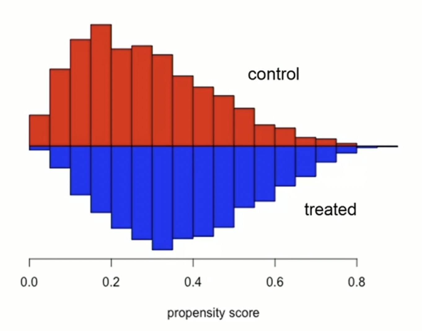
  2. Check that covariates are balanced

     • Usually, we use standardized differences or graphs to examine the distribution of differences

  3. Match each observation in the treatment group to one or more observations in the control group

     • This matching is based on their propensity score

     • Typically, this is done using methods like:

       • Exact matching
       • Caliper matching
       • Nearest neighbor matching
       • Stratification matching
       • Difference-in-differences matching
  4. Verify that covariates are balanced across treatment and control groups
  5. Conduct multivariate analysis based on the new sample

Using Propensity Score Matching

• Typically, a propensity score is esimated by running a logistic regression model

  • Where, the dependent variable is $Z=1$ if the observation is in the treatment group
  • Or, the dependent variable is $Z=0$ if the observation is in the control group
• Specifically, a propensity score represents the propensity of an observation to be in the control group
• Each observations has exactly one propensity score
• Propensity score matching simplifies the matching problem because we only need to match on one variable (propensity score), rather than multiple covariates

• Essentially, the propensity score can be used to check for covariate balance between the treatment group and control group

  • Then, we can say the two groups become observationally equivalent

References

• Wiki about General Procedure of Propensity Score Matching
• Causal Inference Textbook
• Python Causality Handbook
• Comprehensive Causal Inference Textbook
• Paper about the Perils of Propensity Matching