YOLO Algorithm

Improving Accuracy using the YOLO Algorithm

• Now, we have fixed the problem with computational inefficiency
• We still have one problem with our method of object detection
• Specifically, the position of the bounding boxes aren't accurate
• In other words, the position of the bounding boxes are shifted somewhat randomly
• And, the most ideal bounding boxes don't always follow a perfectly squared shape
• We can fix this using the yolo algorithm

Describing the YOLO Algorithm

• The concept of breaking down the images to grid cells is unique in YOLO
• Let's say we have $3 \times 3$ grid

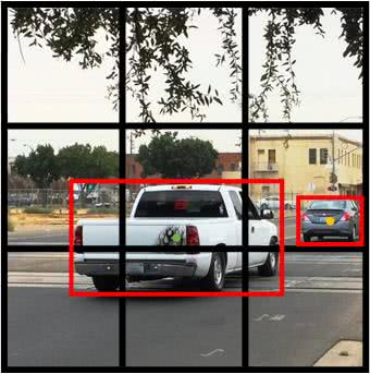
• In the image above we have two cars
• We marked their bounding boxes in red
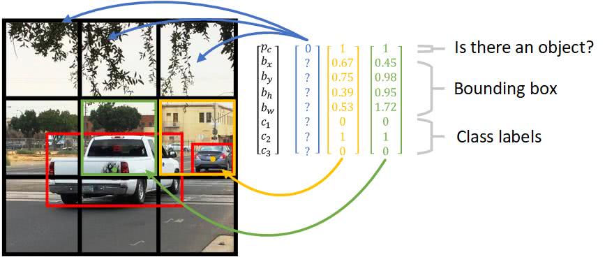
• For each grid cell, we have the following labels for training:

• This is similar to our $1 \times 1$ activations from our convolutional implementation of the sliding window
• Now, we need to associate objects to individual cells
• The rightmost car seems to be obviously associated with the middle-right cell
• The truck seems to be less obviously associated with the center cell
• This is because the yolo algorithm associates an object to a cell based on the object's midpoint

Defining the YOLO Algorithm

• Notice $p_{c}=0$ for cells without objects detected
• We use $?$ because we don't care about its remaining values

• The definition of the bounding box parameters are defined as:

  • $b_{x}:$ The x coordinate corresponding to the center of the bounding box
  • $b_{y}:$ The y coordinate corresponding to the center of the bounding box
  • $b_{h}:$ The height of the bounding box
  • $b_{w}:$ The width of the bounding box
  • $c_{i}:$ The $i^{th}$ class (e.g. pedestrian, car, etc.)
  • $p_{c}:$ The probability of whether there is an object or not
• The yolo loss function is defined as the following:

Intuition behind YOLO Loss Function

• The first term penalizes bad localizations of the center of cells
• The second term penalizes the bounding box with inaccurate height and widths
• The square root is present so that errors in small bounding boxes are more penalizing than erros in big bounding boxes
• The third term tries to make the confidence score equal to the intersection over union between the object and the prediction when there is one object
• The fourth term tries to make the confidence score close to $0$ when there aren't any objects in the cell
• The fifth term is a simple classification loss function

Motivating Nonmax Suppression

• There is still a limitation with our yolo algorithm
• Typically, there are many possible bounding boxes for the yolo algorithm to output
• Specifically, how can we evaluate which bounding box is the best?
• To solve this problem, we'll introduce the concept of nonmax suppression

Introducing Intersection over Union

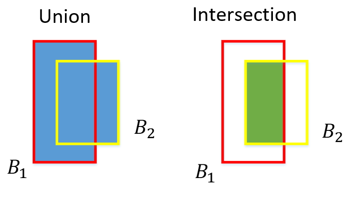
• Before we go into the nonmax suppression concept, we should first introduce the intersection over union (IoU) function
• The iou function is used for evaluating our object detection algorithm
• Specifically, the iou function computes the area of the intersection of two bounding boxes

• The iou function is used for the following:

  • Measuring the similarity of two bounding boxes

  • Training a bounding box against

    • The coordinates of the true bounding box are found manually
    • In other words, we need to be given the coordinates
    • An iou threshold of $0.5$ is considered correct
    • In other words, a bounding box with a $\ge 0.5$ iou value is considered similar enough to the true bounding box

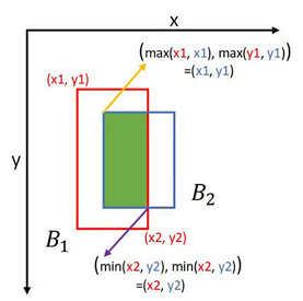
• The iou function doesn't define a bounding box by its center point, width, and height
• Instead, it defines a bounding box based on its upper left corners $(x_{1},y_{1})$ and lower right corners $(x_{2}, y_{2})$

• Specifically, we use the iou function when assigning anchor boxes
• We also use the iou function when assigning anchor boxes

• The algorithm is defined as the following:

  1. Finding the two corners of the intersection
  2. Compute the area of the intersection

def iou(box1, box2):
    xi1 = max(box1[0], box2[0])
    yi1 = max(box1[1], box2[1])
    xi2 = min(box1[2], box2[2])
    yi2 = min(box1[3], box2[3])
    inter_area = (xi2 - xi1) * (yi2 - yi1)

    box1_area = (box1[2] - box1[0]) * (box1[3] - box1[1])
    box2_area = (box2[2] - box2[0]) * (box2[3] - box2[1])
    union_area = box1_area + box2_area - inter_area

    iou = inter_area / union_area

    return iou

Introducing Nonmax Suppression

• Previously, we used a $3 \times 3$ grid to find our bounding boxes
• Realistically, we'll want to use larger grids
• We use larger grids to achieve more accurate bounding boxes
• For example, a $19 \times 19$ grid could be used instead of a $3 \times 3$ grid
• However, we're more likely to pick up multiple bounding boxes for the same object

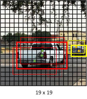
• This is because we're running a localization on each grid
• Therefore, other grids will think there is a car as well

• Our goal is to do the following:

  • Keep the bounding boxes that have the highest $p_{c}$
  • Remove the bounding boxes that are very similar to the bounding boxes with the highest $p_{c}$

• Therefore, we perform nonmax suppression:

  1. Discard all bounding boxes with $p_{c} \le 0.6$
  2. Choose the bounding box with the largest $p_{c}$ value

  3. Discard any remaining boxes with an iou value $\ge 0.5$

     • This is because we want to remove the other similar bounding boxes that aren t the bounding box with the largest $p_{c}$
     • If we removed boxes with an iou value $\le 0.5$, then we'd remove other bounding boxes belonging to other objects

Motivating the Anchor Box

• There is still a limitation with our yolo algorithm
• Let's say we have multiple objects in the same grid cell
• For example, suppose we have a pedestrain and a car in a cell
• Then, do we classify the object as a pedestrian or car?
• To solve this problem, we'll introduce the concept of anchor box

Introducing the Anchor Box

• Anchor boxes allow the yolo algorithm to detect multiple objects centered in one grid cell
• We do this by assigning an additional dimension to the output labels
• This dimension refers to the number of anchor boxes per grid cell
• Meaning, we create another hyperparameter representing the pre-defined number of anchor boxes per cell
• Now, we'll be able to assign one object to each anchor box

Describing Anchor Boxes

• Notice, a car and pedestrian are both centered in the middle cell

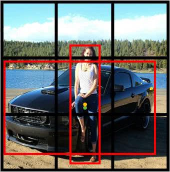
• We should set the number of anchor boxes to be $2$
• Now, each grid cell can detect a pedestrian and a car
• Specifically, a pedestrian and a car in the same cell will be individually assigned to their own anchor box
• This depends on which object and anchor box provide the highest iou value
• Each anchor box specializes in a certain shape
• For example, one anchor box may learn a skinny object, whereas another anchor box may learn a wide object
• In our case, one anchor box could learn a tall, skinny object associated with pedestrians
• And, another anchor box could learn a short, wide object associated with cars
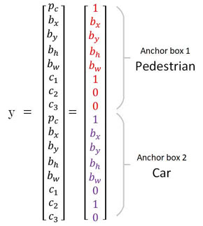
• Our new label will look like the following:

Defining the YOLO Algorithm with Anchor Boxes

• Suppose we are detecting $3$ objects:

  1. Pedestrian
  2. Car
  3. Motorcycle
• Let's also say we're using $2$ anchor boxes per cell
• Lastly, let's say our grid is $3 \times 3$

• Our labels $y$ can be represented as a $3 \times 3 \times 2 \times 8$ matrix:

  • $3 \times 3$ due to the grid size
  • $\times 2$ due to the number of anchors
  • $\times 8$ due to the number of parameters per cell
• Specifically, our label $y_{i}$ can be represented as a $16 \times 1$ vector
• Our label $y_{i}$ looks like the following for a single cell:

• Here $p_{c,1}$ refers to $p_{c}$ of anchor box $1$
• And $p_{c,2}$ refers to $p_{c}$ of anchor box $2$
• Essentially, the yolo algorithm will generate an output matrix of shape $(3,3,2,8)$ given an image
• Meaning, each of the grid cells will output two predictions
• We can observe the dimensions of our labels during the training of a single cell in the image below:

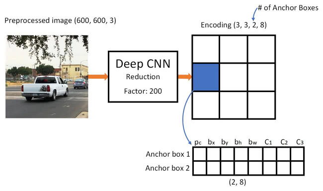
Implementing the YOLO Algorithm with Anchor Boxes

• Let's say we want to train a on the image above
• Specifically, we want to train a convolutional network on the image

• The network will output:

  • A classification of the object
  • A bounding box around the detected object
• An example output of the middle grid cell is the following:

• The output volume $y$ represents a collection of vectors $y_{i}$ associated with one of the $9$ grid cells
• We also need to include nonmax suppresion
• In other words, we'll filter out any improbable bounding boxes
• And, we'll also keep the most probable bounding box associated with an object
• The following image illustrates the generalized steps for predicting objects and their bounding boxes:

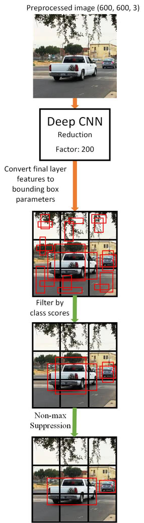
tldr

• The yolo algorithm improves the accuracy of our object detection algorithm

• Specifically, the yolo algorithm is used for accounting for bounding boxes that:

  • May not make up an entire sliding window region
  • May not fall perfectly in an individual grid cell
• In other words, the position of the bounding boxes are shifted somewhat randomly
• The yolo algorithm involves breaking down an image into grid cells

• The definition of the bounding box parameters are defined as:

  • $b_{x}:$ The x coordinate corresponding to the center of the bounding box
  • $b_{y}:$ The y coordinate corresponding to the center of the bounding box
  • $b_{h}:$ The height of the bounding box
  • $b_{w}:$ The width of the bounding box
  • $c_{i}:$ The $i^{th}$ class (e.g. pedestrian, car, etc.)
  • $p_{c}:$ The probability of whether there is an object or not
• The iou function is used for evaluating estimated bounding boxes against the actual bounding boxes
• In other words, the iou function measures the similarity between two bounding boxes
• Nonmax suppression is used for filtering out any bounding boxes that aren't the most probable associated with an object

• Nonmax suppression is defined as the following:

  1. Discard all bounding boxes with $p_{c} \le 0.6$
  2. Choose the bounding box with the largest $p_{c}$ value
  3. Discard any remaining boxes with an iou value $\ge 0.5$
• Anchor boxes allow the yolo algorithm to detect multiple objects centered in one grid cell
• We do this by assigning an additional dimension to the output labels
• This dimension refers to the number of anchor boxes per grid cell
• Meaning, we create another hyperparameter representing the pre-defined number of anchor boxes per cell

References

• Bounding Box Predictions
• Intersection over Union
• Nonmax Suppression
• Anchor Boxes
• Implementing the YOLO Algorithm
• YOLO Object Localization
• Anchor Boxes Chapter
• Defining the YOLO Loss Function
• Illustrating the YOLO Loss Function